
Find the original lab manual here.
Background
Fourier transform is an analysis technique which allows us to observe signal in time domain or its reciprocal domain which is frequency. For this lab we used fast fourier analysis. The difference between the two techniques is computation speed of the algorithm with fft being fast.
Based on the prelab we used the Open Music Labs fft analysis tools. We were focused on analyzing the frequency component of our sound or light signal. The fast fourier analysis allowed us to decompose the time based continuous analog signal into its respective frequency components. From this information, we could easily filter out the range of frequency bins we want to include in our signal. For example, for the acoustic subteam the goal was to detect a 660 Hz signal from the analog singal generated by the microphone. FFT was our tool for the analysis.

The goal of this sublab was to enable our robot to detect a 660hz frequency. In order to do this we had to:
- do a correct FFT analysis,
- have a working amplifier circuit and
- also be able to distinguish a 660 hz from a 585hz and 735 hz.
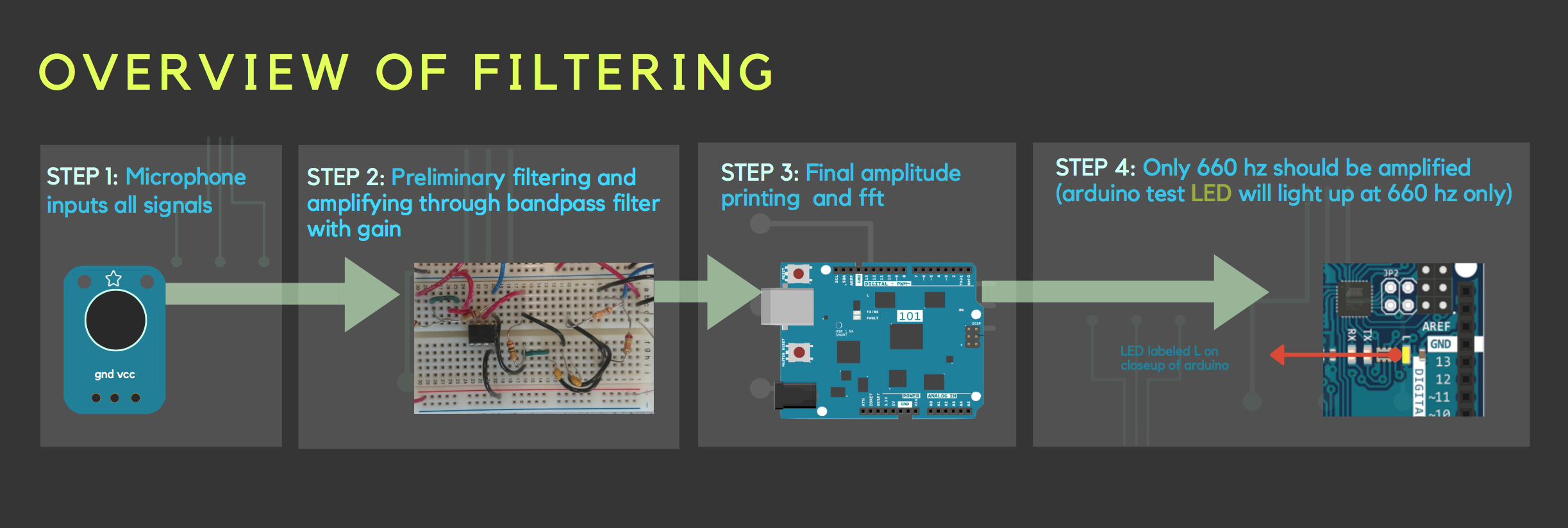
This acoustic aspect of the lab is important because later on the robot will use this 660Hz signal as its start signal. The following is a visual overview of what we want to accomplish
Introduction
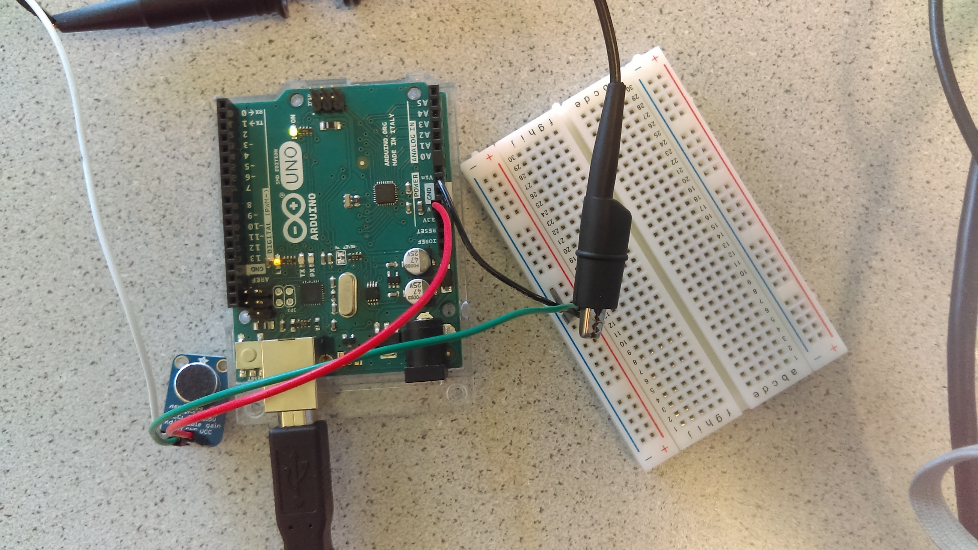
For this lab, we needed a microphone, arduino uno, and some resistors and capacitors. In the past years, the class used a different mic, which is why they previously made a separate microphone circuit. The microphone we used (MAX4466) already came with a low pass filter, which meant that we would not have to do this first step.
First we coded an FFT using the example sketch available in the Open Music Lab library. However, the range of values it provided was still too large to be able to determine the difference between 585, 660, and 735hz satisfactorily. Thus, we created a filter with gain with the dual purpose of narrowing the range and also amplifying. Thus the mic outputs to the filter which then outputs to the arduino and we can interact with the data by printing the values the arduino reads.
To check if the microphone worked properly, we connected it to the arduino and hooked it up to the oscilloscope, turned on a 660hz tone (adjusting the potentiometer on the microphone slightly) and adjusted the scale. In the video, the oscilloscope reads very close to 660 Hz, reconfirming that the microphone is working, and it has read the correct 660hz value we played.
FFT analysis
For this part of the lab we decided to use analogRead. Note that when we use fft_input, each index i that is even represents a real signal, whereas the odd signals are the imaginary components. Thus in the loop:
 for (int i = 0 ; i < 512 ; i += 2) { // save 256 samples
      fft_input[i] = analogRead(A0); // put real data into even bins
      fft_input[i+1] = 0; // set odd bins to 0
We have the the even index 1 equal to the analogRead from pin A0, an i+1 index (the odd one) equal to zero. Then the for loop is incremented by two for each bin.
To check the code and make sure it was working correctly, we hooked it up to the function generator and the oscilloscope to make sure the function generator was outputting as well. We had the arduino print out the values, then we transfered that data to excel and created a bar graph for each bin and signal.
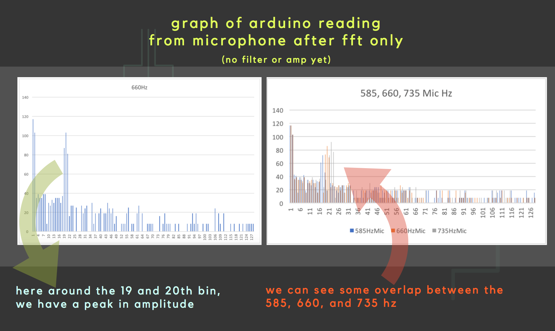
To start off, note first the left bar graph which has a peak in either the 19th or the 20th bin. This is supposed to be around the 17th or 18th, but in our case, it does not change our process or matter that much since everything will be relative, and since we have measured with the oscilloscope that it was recieving the same 660Hz created by the function generator.
We have the other peaks that are the multiples of 660Hz, so that we can be sure the spacing between each peak is equidistant and that the 20 bin number is correct after all.
However, this was not good enough to distinguish from the 585hz and the 735hz. If you look closely at the plot next to it, you can see that the 585hz and 735hz has overlap somewhat with the 660hz. Thus it is necessary for us to further filter and amplify the signal.
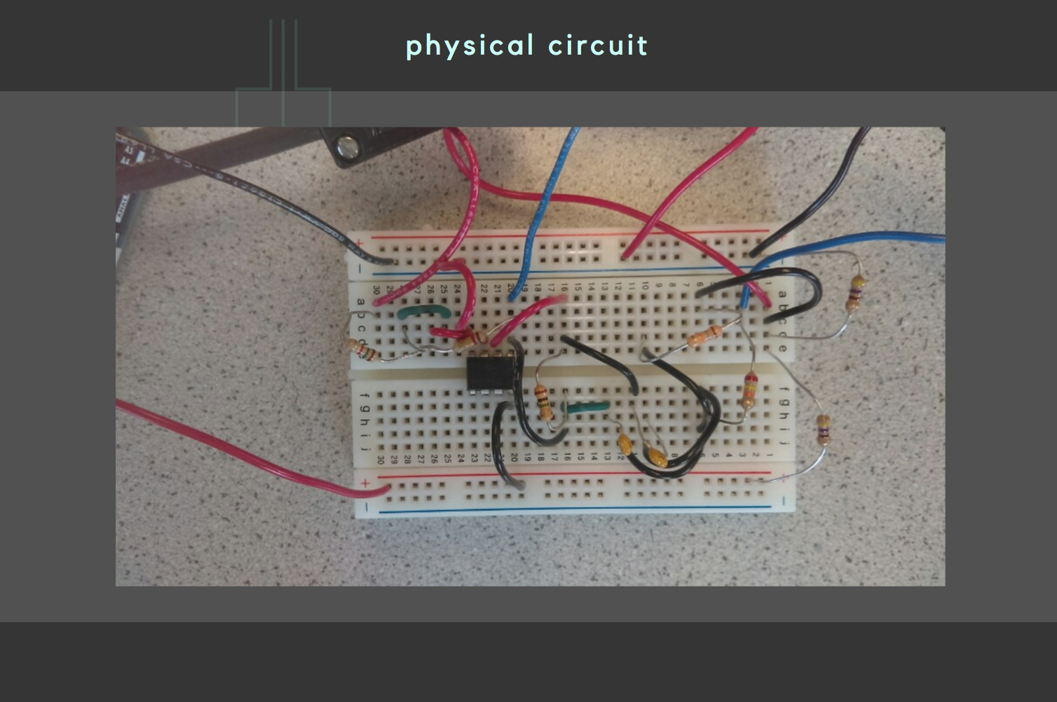
Amplifier Circuit
Rather than making a filter and an amplifier separately, we decided to make a bandpass filter with gain.
Using this website we mapped out what we wanted our Bode plot to look like, such that our 660 Hz signal would be amplified but all others would be minimized. We first started off with a gain of 40db, or 100. The website then outputs a bandpass filter circuit schematic.
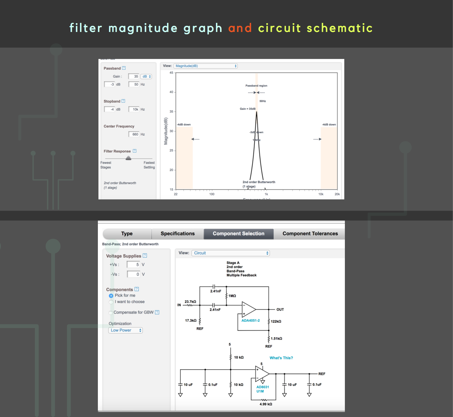
Note that on the website it will output a circuit for voltage range from 5V to -5V, however we want from 5V to 0V. If you change this value, they will give you a REF schematic as well. However this is unnecessary. We simply used a voltage divider to connect the REF and give each 2.5V.
The 2.5 V virtual ground was created by connecting two resistors in parallel. Why did we need to reference our inpur and output resistors to 2.5 volts instead of ground (0 volts)? We did this in order to reduce output swing and gain stability. Our voltage can’t go to negative values. Therefore, using a 2.5 volt as a reference will allow us to swing in the valid voltage ranges. In addition, instead of swinging between 0 and 5 volts, our output now swings between 2.5 and 5 volts.
Distinguishing the 660hz from 585hz and 735hz
In review, the signal that inputs into the microphone gets preliminarily filtered and amplified by our bypass filter with gain. Then the filter outputs into the A0 input pin of the arduino. The arduino code has different amplitudes in each bin, and we can recall that the 660hz amplitude was around the bin 19 and 20. We then added the following code:
    for (byte i = 0 ; i < FFT_N/2 ; i++) {
      Serial.println(fft_log_out[i]); // send out the data
      if (fft_input[38] > 60)
        digitalWrite(LED_BUILTIN, HIGH);
The purpose of this was to be able to show physically that the arduino responded to the 660hz, rather than the 585hz or the 735hz. We did this by making the arduino LED light up when it detected an amplitude higher than 60 in the 19th bin. Recall that the function fft_input allocates two different indexes for each bin, one real and one imaginary. Thus when we want to reference the 19th bin, we actually have to call the 38th as we did in the above code.
You can see in this video that the LED does not light up during the 585 and 735hz tones. This is because we filtered and amplified only the 660hz, so that the amplitude of the 660hz would be the only one with a significantly high amplitude. The 60 value can be adjusted, however we found that our code worked best with the 60.

Introduction The purpose of this part of lab 2 was to enable the Uno to recognize three different frequnecies in IR signals: 7kHz, 12kHz, and 17kHz. A treasure board with ajdustable IR intensity was used as the source for the frequencies, and a phototransistor circuit connected to the Uno was used to detect the frequencies. An Open Music Lab FFT library (as used above) was used to configure relative frequencies into distinct “bins” in order to more feasibly identify different frequencies from one another. Designated bins values were mapped to a range of 0Hz to 0.5*(sampling frequency). V_A3 is measured by the Arduino. This value is measured by the Arduino and FFT analysis is applied. The result is read to the serial monitor as an array of frequency bin amplitudes.
Our IR sensor circuit was connected as follows where the long lead was connected to 5 volts and the other lead was connected to the resistor.
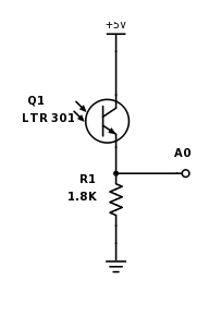
Being that the sensor is NPN phototransistor, this configuration also known as common collector is useful in that it provides slightly less than unity gain but the output impedance is small. The reasoning behind using this configuration over the common emitter amplifier topology is that the common collector circuit allows us to have more control over the gain of the circuit. In testing our circuit, we have found that we do not need an amplifier to detect the IR treasures, but we may still need to make one in the future.
By testing the device at different frequencies, we were able to determine which bins correspond to the frequencies. We used the serial plots to observe which frequencies are affected by the signal.
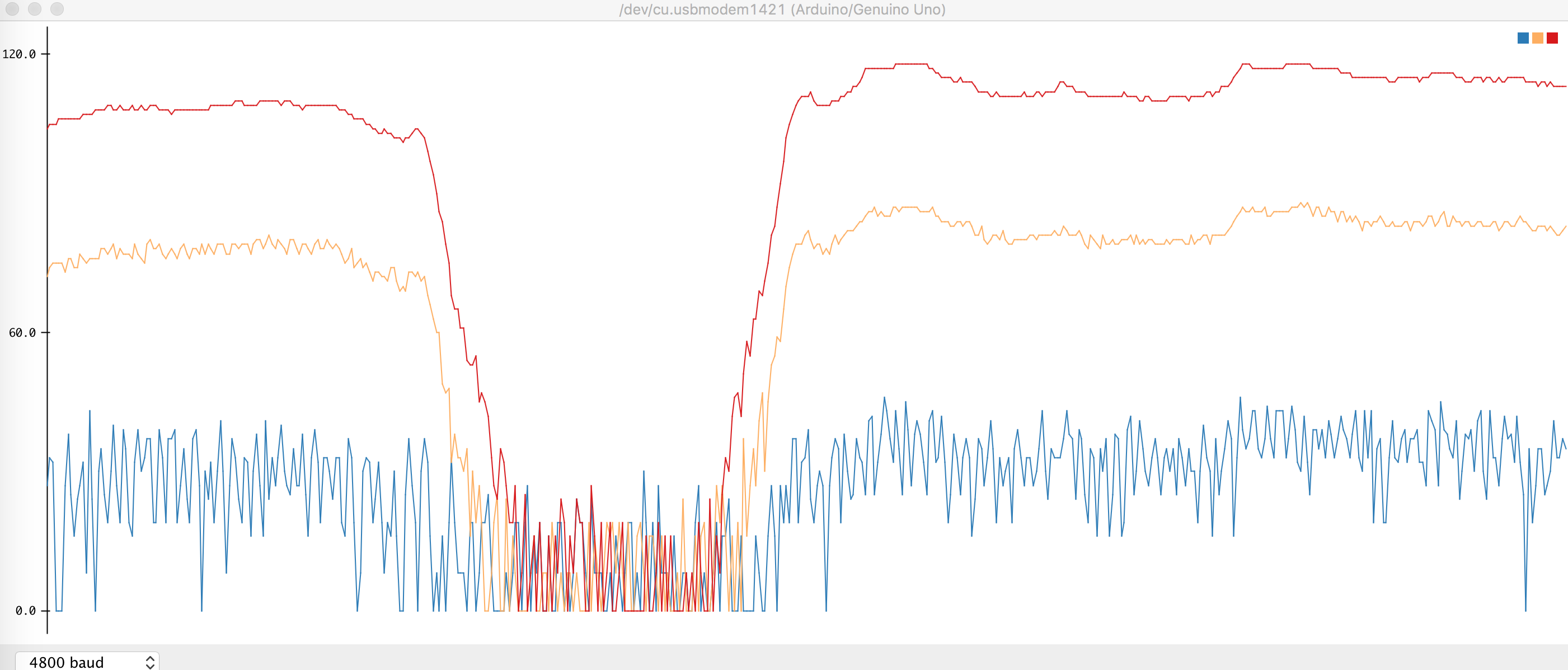 When the signal is applied to the phototransistor, certain frequency bins peak. We took note of these peak bins for different frequency signal inputs and developed an algorithm to detect and output whether the signal is 7kHz, 12kHz, 17 kHz, or none.
| Frequency | Bins |
|---|---|
| 7 kHz | 45, 46, 47 |
| 12 kHz | 79, 80, 81 |
| 17 kHz | 113, 114, 115 |
The reasoning for having a range of bins for each of the frequencies is that that windowing function introduces some frequency smearing between bins.
We designed an algorithm to detect which bins the signals peak at, and how to classify the frequency. Initially, we set a hard FFT cutoff of 70. Values above that threshold were peak values. However, peaks are relative not absolute.
This is how we detect 7 kHz frequencies.
    int range7 = 0;
    for(int i = 10; i < 128; i++){
      if(fft_log_out[i]>60){
        Serial.print(fft_log_out[i]);
        if(i>=45 && i<=47){
          range7++;
        }
    }
There are three integer variables range7, range12, and range17. If all three are zero, there is no signal detected. Otherwise, the greatest integer value is selected. For example, if range7 has the highest non-zero value, a 7 kHz signal is detected.

Since we used two different methods for the FFT, analogRead and the modified free-running sketch from the library, it was fairly easy to merge the code. The only real thing we have to take into consideration is how the loop works.
The acoustic part has to loop until it hears the 660hz after which the loop should end, since the 660hz is only necessary to start the robot. Then we should concentrate our efforts solely on the optical loop, and ignore the acoustic part for the remaining time.